Class 8 Computer Notes for July Month – Navodaya TGT CS

In this article we provide information regarding latest Class 8 Computer Notes for July Month – Navodaya TGT Computer Science (CS) 2024-25.

Class 8 Computer Notes for July Month – Navodaya TGT CS

We are using source for Syllabus – Navodaya Vidyalaya Samiti Perspective Academic Planning Split of Syllabus 2024-25.

We are giving to the Point Notes for the Students.

Thanks Me Later

For the July Month Notes – Class 8 Computer Subject

Unites we covered in Notes

1. Introduction to Excel – 2 (Continued)
   • Changing the width and height of the column and row
   • Finding and select the data in a given range
2. View Menu
   • Gridlines
   • Freeze Panes
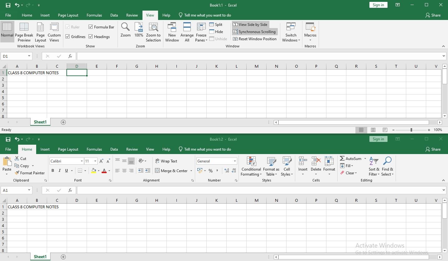
   • View side by side
   • Synchronous scrolling
   • Merging the cells
   • Split the cells

Introduction to Excel – 2 (Continued)

Working with sheets

1. Changing the width and height of the column and row

Resize rows

1. Select a row or a range of rows.
2. On the Home tab, select Format > Row Width (or Row Height).
3. Type the row width and select OK.

Resize columns

1. Select a column or a range of columns.
2. On the Home tab, select Format > Column Width (or Column Height).
3. Type the column width and select OK.

Automatically resize all columns and rows to fit the data

1. Select the Select All button  at the top of the worksheet, to select all columns and rows.
2. Double-click a boundary. All columns or rows resize to fit the data.

2. Finding and Select the Data in a given range

You can quickly locate and select specific cells or ranges by entering their names or cell references in the Name box, which is located to the left of the formula bar:

You can also select named or unnamed cells or ranges by using the Go To (F5 or Ctrl+G) command.

View Menu

1. Gridlines

When you are done with the selection, just navigate to the VIEW tab on the Ribbon and check the Gridlines box in the Show group.

Alternatively, you can go to the Sheet Options group on the PAGE LAYOUT tab and select the View checkbox under Gridlines.

Whichever option you choose gridlines will instantly appear in all the selected worksheets.

2. Freeze panes

Freeze the first column

• Select View > Freeze Panes > Freeze First Column.

            The faint line that appears between Column A and B shows that the first column is frozen.

Freeze the first two columns

1. Select the third column.
2. Select View > Freeze Panes > Freeze Panes.

Freeze columns and rows

1. Select the cell below the rows and to the right of the columns you want to keep visible when you scroll.
2. Select View > Freeze Panes > Freeze Panes.

Unfreeze rows or columns

• On the View tab > Window > Unfreeze Panes.

3. View side by side AND Synchronous scrolling

• Comparing two or more sets of data side by side.
• In Excel, synchronous scrolling allows you to scroll two or more worksheets simultaneously.

View two worksheets in the same workbook side by side in Excel 2007, 2010, 2013 & 2016

1. On the View tab, in the Window group, click New Window.

2. On the View tab, in the Window group, click View Side by Side .
3. In the workbook window, click the worksheets that you want to compare.
4. To scroll both worksheets at the same time, click Synchronous Scrolling in the Window group on the View tab.

 Note   This option is available only when View Side by Side is turned on.

Tips

• If you resize the workbook windows for optimal viewing, you can click Reset Window Position to return to the original settings.
• To restore a workbook window to full size, click Maximize at the upper-right corner of the workbook window.

5. Merging the Cell

Merging combines two or more cells to create a new, larger cell

Home Menu – Alignment Group

Merge cells

1. Select the cells to merge.
2. Select Merge & Center.

Unmerge cells

1. Select the Merge & Center down arrow.
2. Select Unmerge Cells.

6. Split the cell in excel

Split the content from one cell into two or more cells

1. Select the cell or cells whose contents you want to split.
2. Go to Data > Data Tools > Text to Columns.
3. Select the delimiter or delimiters to define the places where you want to split the cell content, and then select Apply.

Thanks to Beloved Readers.